Expectation Maximization is a popular generative algorithm, which elegantly handles Multi-Variate Distributions and tries to find close approximations to underlying data-generating distribution.

For fun, I derived the Multi-Variate Expectation Maximization algorithm, using Mixture of Gaussians. Interested readers can find it here

In following I will consider a particular family of exponential distributions, the Normal Distribution, which for 1-dimensional data x:
$N(x_{n} | \mu_{k}, \sigma^2_{k}) = \frac{1}{\sqrt{2.\pi.\sigma_{k}^2}} . e^\frac{-(x_{n}-\mu_{k})^2}{2.\sigma_{k}^2}$
(subscripts $n \in \{1,2,...N\}\ and\ k \in \{1,2,...K\}$ are for N data points and K Normal Distributions which try to approximate data distribution.
For multidimensional data (s.t. $x_{n}\in \mathbb{R}^D$), Normal Distribution is,
$N(x_{n} | \mu_{k}, \Sigma_{k}) = \frac{1}{\sqrt{det(2.\pi.\Sigma_{k})}}.e^\frac{-(x_{n}-\mu_{k})^T.\Sigma_{k}^{-1}.(x_{n}-\mu_{k})}{2}$
where $\Sigma_{k}$ is covariance matrix for $distribution_{k}$ (or $cluster_{k}$)

For following discussion, we will mainly consider 1-dimensional data x (start from something simple and grow complex!)

EM Algorithm looks like this:

Repeat until convergence:

• find $\gamma_{nk}=\frac{\pi_{k}.N(x_{n}|\mu_{k},\sigma_{k}^2)}{\sum_{k=1}^{K}\pi_{k}.N(x_{n}|\mu_{k},\sigma_{k}^2)}$
  (Can be interpretted as probability of $distribution_{k}$ (or $cluster_{k}$), given data point $x_{n}$ is observed.)

• find $N_{k}=\sum_{n=1}^{N} \gamma_{nk}$
  (Can be interpreted as Expected number of data points which belong to $distribution_{k}$ (or $cluster_{k}$)

• find $\pi_{k}=\frac{N_{k}}{N}$
  (updated prior of the $distribution_{k}$ (or $cluster_{k}$))

• find $\mu_{k}=\frac{\sum_{n=1}^{N} \gamma_{nk}.x_{n}}{N_{k}}$
  (weighted mean of $distribution_{k}$ (or $cluster_{k}$))

• find $\Sigma_{k}=\frac{\sum_{n=1}^{N} \gamma_{nk}.(x_{n}-\mu_{k})(x_{n}-\mu_{k})^T}{N_{k}}$ …[1]
  
  
  Now lets see this algorithm fitting 5-Gaussians (K=5) on a gray-scale image shown below. Size of this image=300KB
  
  
  After running EM algorithm on this image, trying to fit 5-Gaussians, we get following compressed image=100KB
  (Note that actual storage size on disk < 10KB, as this image is actually stored as:

  1. an array of 8 bit integers, each location specifying which cluster it belongs to (that is, most likely Gaussian for that data point).
  2. And only 15 64-bit floating point numbers, with 5 for $\pi$, 5 for $\mu$, 5 for $\sigma^2$.)
     
     
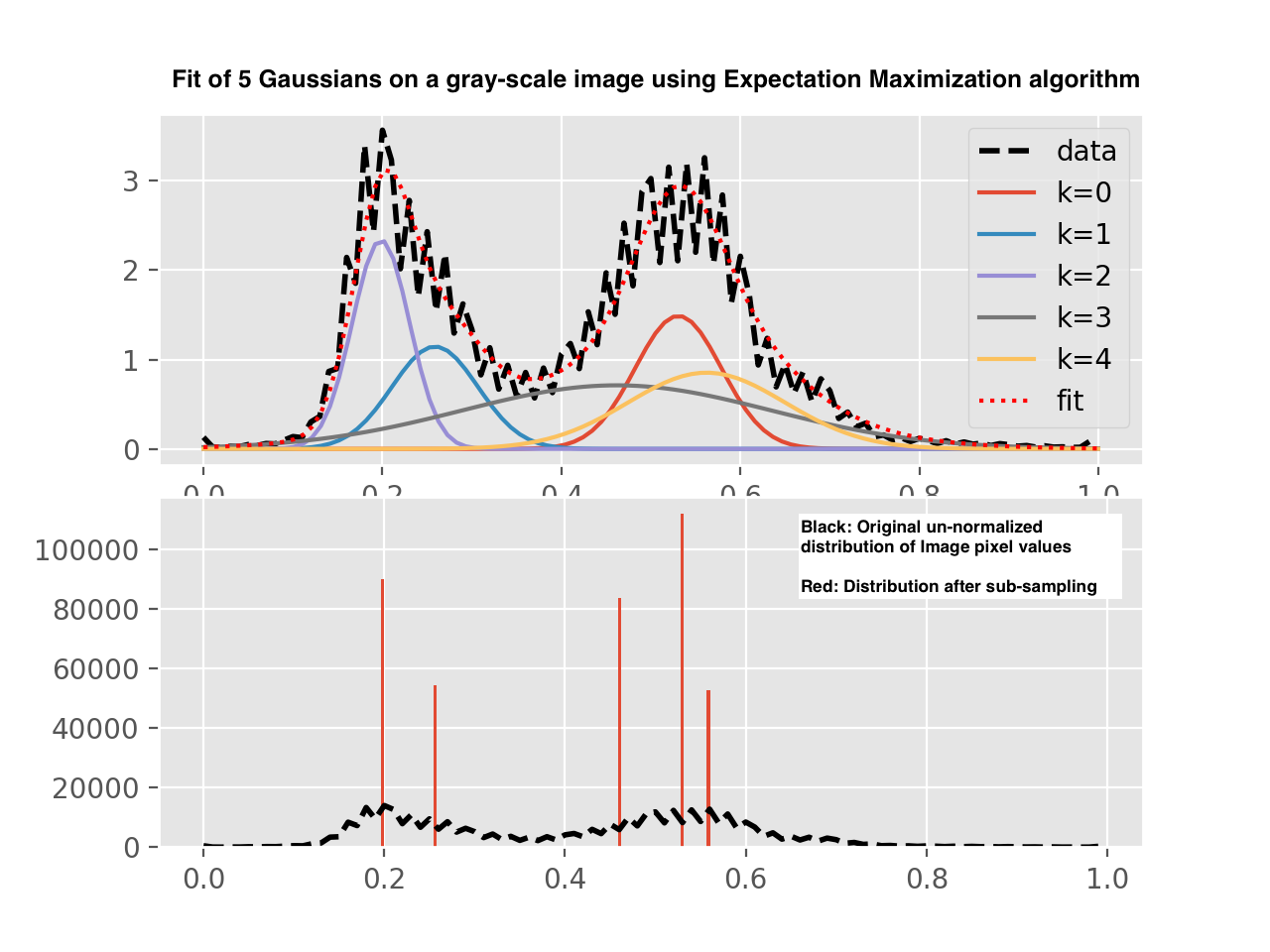
     Following is the statistical analysis of what original image distribution was, how 5-Gaussians were fitted and distribution after sub-sampling to prove that only few unique values are sufficient to describe the compressed image.
     
     
     As seen above, 5-Gaussians fit (Red dotted line in top half) matches closely to actual data distribution. But is of-course a smoothed approximation.
     Bottom-half in picture above compares histogram of sub-sampled image (each pixel value replace with most likely Gaussian), and histogram of original image.
     
     
     
     
     
     
     
     
     
     

     [1]: it is important to interpret $(x_{n}-\mu_{k})(x_{n}-\mu_{k})^T$

     Let us say $x_i \in \mathbb{R}^D$ (and of course also $\mu_{k} \in \mathbb{R}^D$) So, $\begin{bmatrix} x_{i1}-\mu_{k1}\\ x_{i2}-\mu_{k2}\\ ...\\ x_{iD}-\mu_{kD}\\ \end{bmatrix} \times \begin{bmatrix} x_{i1}-\mu_{k1} & x_{i2}-\mu_{k2} & ... & x_{iD}-\mu_{kD}\\ \end{bmatrix}$
     $=\\ \begin{bmatrix}(x_{i1}-\mu_{k1})^2 & (x_{i1}-\mu_{k1})*(x_{i2}-\mu_{k2}) & ... & (x_{i1}-\mu_{k1})*(x_{iD}-\mu_{kD})\\ (x_{i2}-\mu_{k2})*(x_{i1}-\mu_{k1}) & (x_{i2}-\mu_{k2})^2 & ... & (x_{i2}-\mu_{k2})*(x_{iD}-\mu_{kD})\\ ...\\ (x_{iD}-\mu_{kD})*(x_{i1}-\mu_{k1}) & (x_{iD}-\mu_{kD})*(x_{i2}-\mu_{k2}) & ... & (x_{iD}-\mu_{kD})^2\\ \end{bmatrix}$